Beginners Guide to caskade

Here we will introduce all of the relevant concepts and capabilities of caskade and how to build numerical simulators.

import caskade as ck
import torch
import matplotlib.pyplot as plt
import matplotlib.animation as animation
from IPython.display import HTML
from time import time

Basic Template

All caskade simulators follow the same basic template. Certain ingredients are always involved:

• Subclass the Module object

• Call the super().__init__(name) at the top

• Create some Param attributes

• Decorate a function(s) with @forward

• use the params (by name) in the decorated function(s)

You can also provide a name for the Module, though this is optional.

class Gaussian(ck.Module):
    def __init__(self, name, x0=None, q=None, phi=None, sigma=None, I0=None):
        super().__init__(name)
        self.x0 = ck.Param("x0", x0, shape=(2,))  # position
        self.q = ck.Param("q", q)  # axis ratio
        self.phi = ck.Param("phi", phi)  # orientation
        self.sigma = ck.Param("sigma", sigma)  # width
        self.I0 = ck.Param("I0", I0)  # intensity

    @ck.forward
    def _r(self, x, y, x0=None, q=None, phi=None):
        x, y = x - x0[..., 0], y - x0[..., 1]
        s, c = torch.sin(phi), torch.cos(phi)
        x, y = c * x - s * y, s * x + c * y
        return (x**2 + (y * q) ** 2).sqrt()

    @ck.forward
    def brightness(self, x, y, sigma=None, I0=None):
        return I0 * (-self._r(x, y) ** 2 / sigma**2).exp()

We may now create instances of this simulator, and inspect what the compute graph looks like.

firstsim = Gaussian("my_first_module", sigma=0.2, I0=1.0)
print(firstsim)  # print the graph
firstsim.graphviz()  # show the graph

my_first_module|Gaussian
    x0|dynamic
    q|dynamic
    phi|dynamic
    sigma|static: 0.2
    I0|static: 1

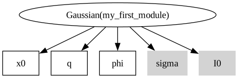
Best practice is to initialize the simulator with initial values for all params (or provide values shortly after creating the simulator as part of initialization).

Use the to_dynamic and to_static to control the status of each param or module.

secondsim = Gaussian("my_second_module", x0=(0, 0), q=0.5, phi=3.14 / 3, sigma=0.2, I0=1.0)
x, y = torch.meshgrid(torch.linspace(-1, 1, 100), torch.linspace(-1, 1, 100), indexing="ij")
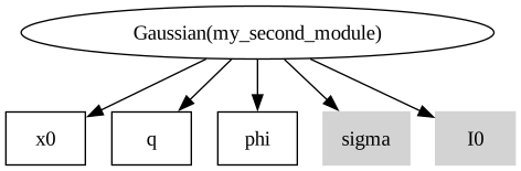
secondsim.to_dynamic()  # all params owned by secondsim are now dynamic
secondsim.sigma.to_static()  # sigma is now static
secondsim.I0.to_static()  # I0 is now static
params = secondsim.get_values()  # automatically build a tensor for the dynamic params
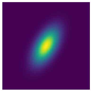
plt.imshow(secondsim.brightness(x, y, params), origin="lower")
plt.axis("off")
plt.show()
secondsim.graphviz()  # show the graph

The parameter order

Since caskade manages the parameters for you, it can automatically build the input tensor with sim.get_values(), but how then do you know what parameter each index corresponds to? This is fairly simple to recover in a few ways depending on the level of detail you want. Let’s explore them here:

# Simplest option, it prints the param names in the order they will be added to the tensor
print(secondsim.param_order())

my_second_module: x0, my_second_module: q, my_second_module: phi

# Most general option, this is the order casakde access the params
print(secondsim.dynamic_params)
# Note that these are the full param objects, so we can access their attributes
print(list(f"{p.name}: {p.npvalue}" for p in secondsim.dynamic_params))
# param.npvalue converts the value into numpy before returning it

(x0, q, phi)
['x0: [0 0]', 'q: 0.5', 'phi: 1.0466666221618652']

caskade collapses all params into a 1D array, even if the param had multiple values itself. To explore the 1D array you can use the “finders” as shown below.

params = secondsim.get_values()
print(params)
# Hmmm, I wonder which param goes in place 3?
# The result is a tuple (Param, index), the index tells you within the param
# where the index 3 lands. Since phi is a scalar this is just ()
print(secondsim.find_param(3))
# Notice if we get index 1 the returned index is more interesting
print(secondsim.find_param(1))

# Hmmm, I wonder which index the q param corresponds to?
print(secondsim.find_index(secondsim.q))
# For multidimensional params, we will get a slice instead
print(secondsim.find_index(secondsim.x0))

# You can also query lists to get a bunch at once
print(secondsim.find_param([0, 1, 2]))

tensor([0.0000, 0.0000, 0.5000, 1.0467])
(phi, ())
(x0, (1,))
2
slice(0, 2, None)
((x0, (0,)), (x0, (1,)), (q, ()))

Different ways to pass the parameters

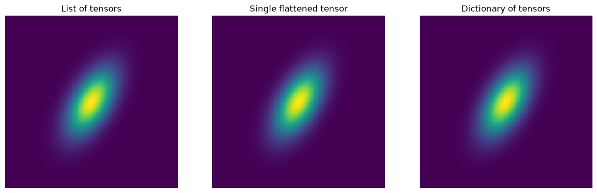
W can pass the parameters into a caskade forward method as one of a list, a 1D Tensor, or a dict.

fig, ax = plt.subplots(1, 3, figsize=(15, 5))
# List of tensors
params_list = secondsim.get_values("list")
print("Params list:", params_list)
ax[0].imshow(secondsim.brightness(x, y, params_list), origin="lower")
ax[0].axis("off")
ax[0].set_title("List of tensors")

# Single flattened tensor
params_tensor = secondsim.get_values("array")
print("Params tensor:", params_tensor)
ax[1].imshow(secondsim.brightness(x, y, params_tensor), origin="lower")
ax[1].axis("off")
ax[1].set_title("Single flattened tensor")

# Dictionary of tensors, using attribute names of either Param or Module objects
params_dict = secondsim.get_values("dict")
print("Params dict:", params_dict)
ax[2].imshow(secondsim.brightness(x, y, params_dict), origin="lower")
ax[2].axis("off")
ax[2].set_title("Dictionary of tensors")
plt.show()

Params list: [tensor([0, 0]), tensor(0.5000), tensor(1.0467)]
Params tensor: tensor([0.0000, 0.0000, 0.5000, 1.0467])
Params dict: {'x0': tensor([0, 0]), 'q': tensor(0.5000), 'phi': tensor(1.0467)}

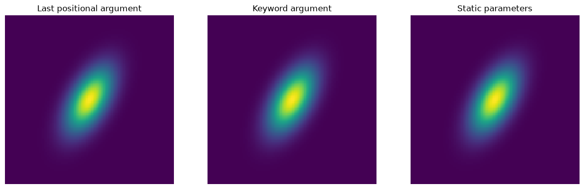
Next, once we have the params we can either pass it as the last positional argument, as a params= keyword, or we can set them as static.

fig, ax = plt.subplots(1, 3, figsize=(15, 5))

# Pass as last positional argument
ax[0].imshow(secondsim.brightness(x, y, params_list), origin="lower")
ax[0].axis("off")
ax[0].set_title("Last positional argument")

# Pass as keyword argument
ax[1].imshow(secondsim.brightness(x, y, params=params_list), origin="lower")
ax[1].axis("off")
ax[1].set_title("Keyword argument")

# Set parameters as static
secondsim.to_static()
ax[2].imshow(secondsim.brightness(x, y), origin="lower")
ax[2].axis("off")
ax[2].set_title("Static parameters")
# Set them back to dynamic
secondsim.x0.to_dynamic()
secondsim.q.to_dynamic()
secondsim.phi.to_dynamic()
plt.show()

Update values in simulator

As we run sampling and optimization, we will want to change the stored values in the simulator. While you can update them individually with param.value = new_value there are also efficient ways of updating the parameters using the same format as getting the parameters!

current_values = secondsim.get_values()
# something like: new_values = scipy.optimize.minimize(secondsim.likelihood, current_values).x
new_values = current_values
secondsim.set_values(new_values)  # Yay, it's now updated.
# This will work for array, list, or dict formats

The pointer parameter

So far we have only looked at dynamic and static parameters. caskade allows users to build complex simulators with relationships between parameters. Next lets see the pointer type:

• dynamic is given as input when calling a @forward method

• static is a fixed value

• pointer returns the value computed from other nodes in the graph

thirdsim = Gaussian("my_third_module", phi=3.14 * 5 / 6, q=0.2, sigma=0.2, I0=0.5)
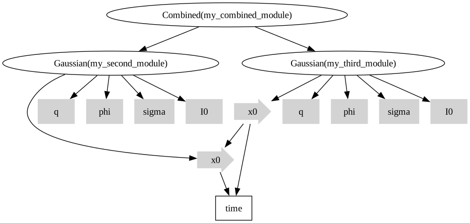
thirdsim.x0 = secondsim.x0  # now they share the same position

thirdsim.graphviz()

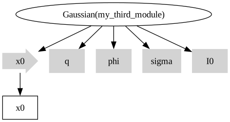
As you can see, a pointer parameter is represented in the graph as a shaded arrow. It will now return the same value as the x0 parameter in secondsim.

Linking and unlinking params

Pointer parameters can be linked to and unlinked from other nodes. Use link(node) to connect a child node, and unlink(node) (or a key string) to disconnect a specific child. Calling unlink() with no arguments removes all children at once, acting as a convenient clear.

time_param = ck.Param("mytime")  # a standalone param to link against
shared_x0 = ck.Param("shared_x0", shape=(2,))

# Link a child node using a key or by passing the node directly
shared_x0.link("mytime", time_param)
print("Children after link:", list(shared_x0.children))

# Unlink a specific child by key or node reference
shared_x0.unlink("mytime")
print("Children after unlink(key):", list(shared_x0.children))

# Re-link and then clear all children at once
shared_x0.link("mytime", time_param)
shared_x0.unlink()  # removes all children
print("Children after unlink():", list(shared_x0.children))

Children after link: ['mytime']
Children after unlink(key): []
Children after unlink(): []

Nested Modules

The real power of caskade comes from nesting Module objects to build complex scientific simulators, all while keeping the flexible and robust interfaces seen above.

class Combined(ck.Module):
    def __init__(self, name, first, second):
        super().__init__(name)
        self.first = first  # Modules are automatically registered
        self.second = second

    @ck.forward
    def brightness(self, x, y):
        return self.first.brightness(x, y) + self.second.brightness(x, y)

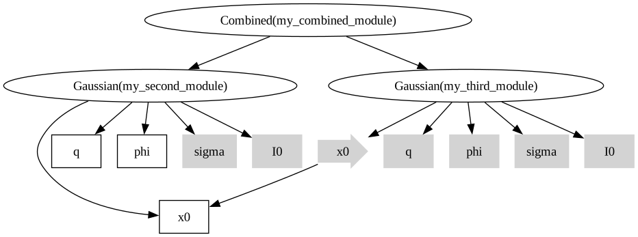
combinedsim = Combined("my_combined_module", secondsim, thirdsim)
print(combinedsim)
combinedsim.graphviz()

my_combined_module|Combined
    my_second_module|Gaussian
        x0|dynamic: [0, 0]
        q|dynamic: 0.5
        phi|dynamic: 1.05
        sigma|static: 0.2
        I0|static: 1
    my_third_module|Gaussian
        x0|pointer: [0, 0]
            x0|dynamic: [0, 0]
        q|static: 0.2
        phi|static: 2.62
        sigma|static: 0.2
        I0|static: 0.5

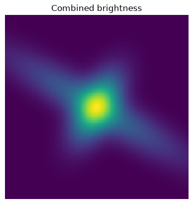
# same params as before since secondsim is all static or pointers to firstsim
plt.imshow(combinedsim.brightness(x, y, combinedsim.get_values()), origin="lower")
plt.axis("off")
plt.title("Combined brightness")
plt.show()

Functional pointers

A pointer parameter determines it’s value from other parameters. This can go beyond just returning the same value. One can define an arbitrary function.

simtime = ck.Param("time")  # create a parameter for time
secondsim.x0 = lambda p: (-p.time.value + 0.5) * torch.tensor((1, -1))
secondsim.x0.link(simtime)
thirdsim.x0 = lambda p: p.time.value * torch.tensor((1, 1)) - 0.5
thirdsim.x0.link(simtime)

# Use `to_static(value)` to set the value and set to static
# Similarly use `to_dynamic(value)` to set value and set dynamic
secondsim.q.to_static(0.5)
secondsim.phi.to_static(3.14 / 3)

combinedsim.graphviz()

Show code cell source

Hide code cell source

B = 64
fig, ax = plt.subplots()
img = ax.imshow(combinedsim.brightness(x, y, torch.tensor([0.0])), origin="lower", vmin=0, vmax=1.5)
ax.set_title("Brightness at time 0")


def update(i):
    img.set_data(combinedsim.brightness(x, y, torch.tensor([i / B])))
    ax.set_title(f"Brightness at time {i / B:.2f}")
    return img


ani = animation.FuncAnimation(fig, update, frames=B, interval=60)

plt.close()

# Or display the animation inline
HTML(ani.to_jshtml())

Once Loop Reflect

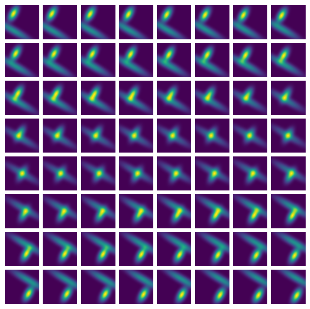
Interacting with PyTorch

The above animation was made with a for-loop, but using the PyTorch vmap function we can produce the frames a lot faster. In this case, vmap is up to 5x faster than the for-loop but with lots of fluctuations.

batched_params_tensor = torch.linspace(0, 1, 64).reshape(
    64, 1
)  # only 1 param "time" so last dim is 1

start = time()
result = []
for i in range(B):
    result.append(combinedsim.brightness(x, y, batched_params_tensor[i]))
result = torch.stack(result)
print("for-loop time taken: ", time() - start)

vbrightness = torch.vmap(combinedsim.brightness, in_dims=(None, None, 0))
start = time()
result = vbrightness(x, y, batched_params_tensor)
print("vmap time taken: ", time() - start)

for-loop time taken:  0.028057575225830078
vmap time taken:  0.027979135513305664

Show code cell source

Hide code cell source

fig, axarr = plt.subplots(8, 8, figsize=(8, 8))
plt.subplots_adjust(wspace=0.1, hspace=0.1)
for i, ax in enumerate(axarr.flat):
    ax.imshow(result[i], origin="lower")
    ax.axis("off")
plt.show()

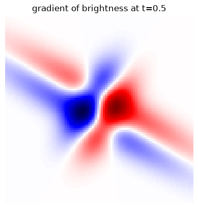
We can also use PyTorch autograd functionalities on caskade simulators. All of the PyTorch calculus operations will work on caskade simulators, so one may compute a likelihood and perform gradient descent very easily, to name one example.

# using PyTorch autograd
params_tensor = torch.tensor([0.5])
plt.imshow(
    torch.func.jacfwd(combinedsim.brightness, argnums=2)(x, y, params_tensor),
    origin="lower",
    cmap="seismic",
)
plt.axis("off")
plt.title("gradient of brightness at t=0.5")
plt.show()

Use caskade with numpy, JAX, or PyTorch

It is possible to use caskade with other array like types like numpy and jax. You’ll need to set the backend for caskade to run things properly. Ideally you should set the environment variable CASKADE_BACKEND and then caskade will run everything with your desired backend. The options are torch, numpy, and jax. If you have a linux system running bash you can do:

export CASKADE_BACKEND="numpy"

to switch over to run everything with numpy, and similar commands for any other backend option. The default is torch since that’s what caskade was originally developed in. You can also change the backend on the fly like below, just note that this is a bit dangerous since you can have objects running around with different types. Ideally, you would set the backend at the top of your script and leave it as the same value throughout.

# numpy backend
ck.backend.backend = "numpy"
p = ck.Param("p", 1.0)
print("with numpy backend, p type:", type(p.value))

# jax backend
ck.backend.backend = "jax"
p = ck.Param("p", 1.0)
print("with jax backend, p type:", type(p.value))

# torch backend
ck.backend.backend = "torch"
p = ck.Param("p", 1.0)
print("with torch backend, p type:", type(p.value))

with numpy backend, p type: <class 'numpy.ndarray'>

with jax backend, p type: <class 'jaxlib._jax.ArrayImpl'>
with torch backend, p type: <class 'torch.Tensor'>

And we’re done! Those are all the elemental abilities of caskade, I hope that by this point you have a sense of the vast possibilities of simulators that can be constructed. This is only the tip of the iceberg for caskade, check out the advanced tutorial for much more information about constructing simulators! Or check out caustics to see caskade in action!

Happy science-ing!